The Discrete Fourier Transform, From Scratch

If you’ve worked with signals before, you’ve likely heard Fourier transforms come up a lot. The goal of this post is to work through what they actually do, starting with a question about sound:

If I take a block of samples from an audio waveform, how can I figure out which frequencies make up those samples?

The tool we’ll use is the Discrete Fourier Transform, or DFT. For now, think of it as a black box. We feed in a few thousand samples and get back a list of complex numbers called frequency coefficients. Each coefficient measures the contribution of one particular frequency to the block.

But what does it mean for a frequency to be “in” a waveform? Imagine adding a strong $440$ Hz cosine wave to a weaker $880$ Hz cosine wave, point by point. The resulting waveform has a more complicated shape, even though we made it from two simple repeating patterns. Sine and cosine waves are collectively called sinusoids. The DFT lets us work backwards from the samples of that combined waveform to its sinusoidal components.

There are a few things to unpack here. Why are the output numbers complex when the input samples are real? How does a number describe a frequency? And how much can a finite set of samples tell us about the original continuous sound? That last question matters: the DFT gives us an exact description of the samples, but interpreting them as evidence about the original sound requires some care.

I want to work through the math closely enough that each part of the formula has a reason to be there. We’ll start with how sound becomes numbers, build up the frequency tests, then calculate a complete DFT by hand. The example uses only four samples so we can see every multiplication, including where magnitude and phase come from.

1. From sound to samples

From air pressure to a list of numbers

When you speak, the air pressure near a microphone changes over time. We model those changes as a continuous-time signal: a function with a value at every instant, including the instants when nobody measures it.

A microphone converts the pressure changes into a changing electrical voltage. An analog-to-digital converter (ADC) samples that voltage at evenly spaced times and rounds each measurement to one of its available digital values:

$$\text{air pressure} \longrightarrow \text{microphone voltage} \longrightarrow \text{digital samples}.$$

Let’s call the voltage signal $x(t)$. To keep the math simple, we’ll ignore the ADC’s rounding for now. If we take $f_s$ samples per second, then the time between measurements is

$$T_s = \frac{1}{f_s}\text{ seconds}.$$

This $f_s$ is the sampling rate. For example, $f_s=1{,}000$ means one measurement every $1/1{,}000$ of a second. We number the samples starting at zero, so sample $n$ is taken at

$$t_n = nT_s = \frac{n}{f_s}.$$

We use square brackets to distinguish a sample index from a time in seconds. The value at index $n$ is just the continuous signal evaluated at that sample’s time:

$$x[n] = x\left(\frac{n}{f_s}\right).$$

Each $x[n]$ is an ordinary real number. A positive or negative value says which side of the waveform’s zero level we’re on; its size says how far away we are. The DFT can also take complex inputs, but we’ll start with these real audio samples. Pick a finite block containing $N$ of them:

$$x[0],x[1],\ldots,x[N-1].$$

These values can be anything. A recording of speech doesn’t have to look like a neat cosine wave for the DFT to work. The sinusoids are the patterns we’ll use to describe the samples, not a requirement we impose on the input.

So what does the DFT give us in place of this list?

The same samples in new coordinates

I’ll put the formula here so we have something to come back to:

$$X[k] = \sum_{n=0}^{N-1} x[n]e^{-j2\pi kn/N}, \qquad k=0,1,\ldots,N-1.$$

We haven’t defined the exponential yet. Set that aside for a moment and look at the input and output sizes:

$$\underbrace{x[0],x[1],\ldots,x[N-1]}_{N\text{ time-domain samples}} \quad\xrightarrow{\text{DFT}}\quad \underbrace{X[0],X[1],\ldots,X[N-1]}_{N\text{ frequency coefficients}}.$$

The lowercase $x$ describes the signal in the time domain: what was its value at each sampled moment? The uppercase $X$ describes it in the frequency domain: how much of each candidate sinusoid do we need, and where in its cycle should it start? The index $n$ picks a sample; the index $k$ picks a frequency coefficient.

We’re still describing the same $N$ samples. If we keep the full complex coefficients, the inverse DFT can recover every one of them. Think of describing a location by its horizontal and vertical offsets, or by its distance and direction from you. The description changes, but the location doesn’t.

Before we unpack those complex numbers, there’s a naming distinction worth making. The DFT is one member of a larger family of Fourier tools.

Where the DFT fits in Fourier analysis

You may have heard that “any signal is a sum of sines and cosines.” That’s useful intuition, but the precise statement depends on the kind of signal we’re describing:

Tool	Input	Frequency description	Example
Fourier series	Continuous-time and periodic	Discrete frequencies	An ideal square wave repeating forever
Fourier transform	Continuous-time, including non-periodic signals	Continuous frequency variable	One isolated acoustic pulse
Discrete-Time Fourier Transform (DTFT)	Discrete-time, finite or infinite sequence	Continuous, periodic frequency variable	An infinite decaying sequence
DFT	Discrete-time, finite block	$N$ discrete frequency bins	A block of 1,024 audio samples

For a suitable periodic continuous-time signal, a Fourier series uses a possibly infinite sum of sinusoids. For suitable non-periodic signals, the inverse Fourier transform uses an integral over frequencies instead. The conditions for those continuous-time results are beyond what we need here. The finite DFT has a particularly convenient guarantee: any list of $N$ numbers can be written as a combination of its $N$ basis sequences. We’ll see why that works below.

First, we need to understand the expression $e^{j\theta}$. Everything after that will use the same picture of a point on a circle.

2. From a complex point to a sinusoid

A point on the complex plane

An ordinary real number tells us where we are on a number line. To plot a complex number, we add a second axis at right angles to the first. This gives us the complex plane:

• The horizontal axis is the real axis.
• The vertical axis is the imaginary axis.

Signal processing usually writes the imaginary unit as $j$ because $i$ is often reserved for electric current. Its defining property is

$$j^2=-1.$$

A complex number has the form

$$z=a+bj,$$

where $a$ and $b$ are ordinary real numbers. On the complex plane, $z$ is simply the point $(a,b)$. Move $a$ units horizontally and $b$ units vertically.

For example, $3+2j$ is the point $(3,2)$.

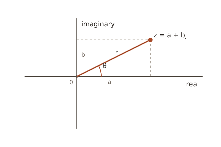
The arrow from the origin to this point has a length

$$r=|z|=\sqrt{a^2+b^2}$$

and an angle

$$\theta=\operatorname{atan2}(b,a).$$

The length comes from Pythagoras. The angle needs a little more care: taking $\arctan(b/a)$ alone can’t distinguish, for example, $(1,1)$ from $(-1,-1)$. The function $\operatorname{atan2}(b,a)$ uses the signs of both coordinates to choose the right quadrant. We measure angles counterclockwise from the positive real axis, with a full turn equal to $2\pi$ radians.

If $z=0$, the arrow has no length and therefore no defined direction. Every nonzero complex number has both a magnitude and an angle.

Draw a right triangle from the arrow to the horizontal axis. Cosine gives the horizontal coordinate divided by the radius, and sine gives the vertical coordinate divided by the radius. Rearranging,

$$\begin{aligned} a &= r\cos(\theta),\\ b &= r\sin(\theta). \end{aligned}$$

Substitute these coordinates into $z=a+bj$:

$$z=r\cos(\theta)+jr\sin(\theta) =r\bigl(\cos(\theta)+j\sin(\theta)\bigr).$$

We now have two descriptions of the same complex number:

• Cartesian form: $a+bj$ gives horizontal and vertical coordinates.
• Polar form: $r$ and $\theta$ give length and direction.

That expression inside the parentheses has another name: $e^{j\theta}$. Let’s see where it comes from.

Euler’s formula

Euler’s formula says

$$e^{j\theta}=\cos(\theta)+j\sin(\theta).$$

All angles in what follows are measured in radians.

At first glance, exponentials and circles don’t seem particularly related. Why should raising $e$ to an imaginary power give us those two coordinates?

We can work it out using Taylor series. These express a function as a sum of powers of its input, with coefficients determined by its derivatives at a chosen point. For the exponential, cosine, and sine, the series about zero are

$$\begin{aligned} e^x &= 1+x+\frac{x^2}{2!}+\frac{x^3}{3!}+\frac{x^4}{4!}+\cdots,\\ \cos(x) &= 1-\frac{x^2}{2!}+\frac{x^4}{4!}-\cdots,\\ \sin(x) &= x-\frac{x^3}{3!}+\frac{x^5}{5!}-\cdots. \end{aligned}$$

Here $3!$, for example, means $3\times2\times1$. These particular series converge for every real or complex input, so we can use the exponential series to define $e^z$ for complex $z$. Replace $x$ with $j\theta$:

$$e^{j\theta} =1+j\theta+\frac{(j\theta)^2}{2!} +\frac{(j\theta)^3}{3!} +\frac{(j\theta)^4}{4!}+\cdots.$$

The powers of $j$ repeat every four steps:

$$j^0=1,\qquad j^1=j,\qquad j^2=-1,\qquad j^3=-j,\qquad j^4=1.$$

Use that cycle and group the real and imaginary terms:

$$\begin{aligned} e^{j\theta} &=\left(1-\frac{\theta^2}{2!}+\frac{\theta^4}{4!}-\cdots\right)\\ &\quad+j\left(\theta-\frac{\theta^3}{3!}+\frac{\theta^5}{5!}-\cdots\right)\\ &=\cos(\theta)+j\sin(\theta). \end{aligned}$$

Look back at the two series in parentheses. The first is exactly the Taylor series for cosine, and the second is exactly the one for sine. The powers of $j$ supplied all the alternating signs we needed. Since the series converge absolutely, grouping the terms this way is valid.

It lets us rewrite the polar form of any complex number as

$$\boxed{z=re^{j\theta}}.$$

The magnitude $r$ is the arrow’s length. The angle $\theta$ is its direction.

A fixed angle is a point; a changing angle is rotation

For one fixed value of $\theta$, $e^{j\theta}$ is one point:

$$e^{j\theta} =\underbrace{\cos(\theta)}_{\text{horizontal coordinate}} +j\underbrace{\sin(\theta)}_{\text{vertical coordinate}}.$$

Its distance from the origin is always one because

$$\cos^2(\theta)+\sin^2(\theta)=1.$$

That is why these points lie on the unit circle.

Rotation appears only when $\theta$ changes. As the angle increases, the point visits familiar positions:

Angle	Complex point	Position
$0$	$1+j0$	Right
$\pi/2$	$0+j$	Top
$\pi$	$-1+j0$	Left
$3\pi/2$	$0-j$	Bottom
$2\pi$	$1+j0$	Back to the start

One complete turn is $2\pi$ radians.

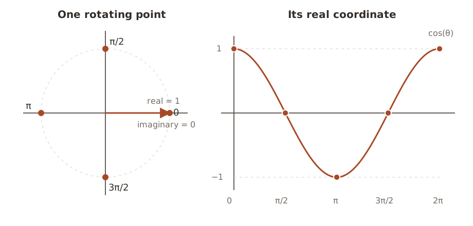
In the figure, we’re plotting the arrow’s horizontal coordinate against angle. At angle zero that coordinate is $1$. A quarter-turn later it’s $0$, halfway around it’s $-1$, and eventually it returns to $1$. That’s the cosine wave. Following the vertical coordinate instead gives us sine.

Make the angle change with time

Frequency $f$ measures cycles per second. Since one cycle contains $2\pi$ radians, a point rotating at $f$ cycles per second moves

$$\omega=2\pi f$$

radians per second. The symbol $\omega$ is called angular frequency.

If we start at angle zero, then after $t$ seconds the point has moved

$$\theta(t)=\omega t=2\pi ft$$

radians. If it starts at some angle $\phi$, then

$$\theta(t)=2\pi ft+\phi.$$

If we also allow the circle to have radius $A\geq0$, we get

$$\boxed{z(t)=Ae^{j(2\pi ft+\phi)}}.$$

Its three parameters have concrete meanings:

• $A$ is the amplitude. On the complex plane, it is the circle’s radius.
• $f$ is the frequency in cycles per second, or hertz.
• $\phi$ is the initial phase. It is the starting angle at $t=0$.

Euler’s formula separates its coordinates:

$$z(t)=A\cos(2\pi ft+\phi)+jA\sin(2\pi ft+\phi).$$

Note that “phase” can refer to two related things here:

• $\phi$ is the initial phase. It stays fixed.
• $2\pi ft+\phi$ is the current angle, sometimes called the instantaneous phase in this simple constant-frequency case. It changes with time.

For example, set $f=1$ Hz and $\phi=0$. At $t=1/4$ second, the current angle is $2\pi(1)(1/4)=\pi/2$. The initial phase is still zero; it describes where we started, not where we are now. As with any angle around a circle, adding $2\pi$ gives the same position.

Why keep the imaginary coordinate?

A physical audio waveform is real-valued. If we want the real cosine

$$x(t)=A\cos(2\pi ft+\phi),$$

we can obtain it as the real-coordinate projection of the complex rotation:

$$x(t)=\operatorname{Re}\left\{Ae^{j(2\pi ft+\phi)}\right\}.$$

The operator $\operatorname{Re}$ means “take the real part.” For plotting or playing this known cosine, that’s all we need. The imaginary sine isn’t another physical signal hiding in the microphone recording. We chose to introduce it when we represented the cosine using a point on a circle.

So what does keeping that extra coordinate buy us?

At a single instant, a cosine value does not tell us the point’s full position in its cycle. Both

$$\cos\left(\frac{\pi}{2}\right)=0 \qquad\text{and}\qquad \cos\left(\frac{3\pi}{2}\right)=0.$$

The real coordinate is zero in both cases. The imaginary coordinate distinguishes them:

$$e^{j\pi/2}=+j, \qquad e^{j3\pi/2}=-j.$$

If the point is rotating counterclockwise, $+j$ is where its real coordinate crosses zero going downward, while $-j$ is where it crosses going upward. The extra coordinate distinguishes those positions. One point alone doesn’t tell us the direction of motion; here we know it from our choice of positive frequency.

But we started with a known cosine. In an actual recording, we don’t know the sinusoid’s phase ahead of time. Suppose we try to find a frequency by comparing the samples with a cosine at that frequency. Could a sine at the same frequency go undetected?

Take four samples of one cosine cycle and one sine cycle:

$$c=[1,0,-1,0], \qquad s=[0,1,0,-1].$$

One way to compare two lists is to multiply corresponding entries and add the results. This is their dot product. Matching signs make positive contributions; opposite signs make negative contributions. For these two lists,

$$c\cdot s=1(0)+0(1)+(-1)(0)+0(-1)=0.$$

The score is zero, despite the waves having the same frequency. Now compare the sine with itself:

$$s\cdot s=0(0)+1(1)+0(0)+(-1)(-1)=2.$$

The sine reference catches what the cosine reference missed. Both tests are useful because we don’t know where the wave starts in its cycle.

The DFT keeps both scores in one complex number: the cosine score is its real coordinate, and the negative sine score is its imaginary coordinate. We’ll derive that minus sign shortly. The number’s length combines the two scores, and its angle tells us how they’re divided. That’s how we’ll recover amplitude and phase.

This also explains why real audio samples can produce complex output. We’re making two measurements from the same real list. Before combining those measurements into the DFT, we need to express our sinusoids at the sample times.

3. From sinusoids to the DFT

Move from continuous time to sample number

We already worked out when sample $n$ is taken:

$$t_n=\frac{n}{f_s}.$$

So there’s no new kind of sinusoid to invent. Substitute $t=n/f_s$ into the one we already have:

$$\begin{aligned} z[n] &=Ae^{j(2\pi f(n/f_s)+\phi)}\\ &=Ae^{j(2\pi(f/f_s)n+\phi)}. \end{aligned}$$

The ratio

$$\frac{f}{f_s}$$

has units of cycles per sample:

$$\frac{\text{cycles}}{\text{second}} \div \frac{\text{samples}}{\text{second}} = \frac{\text{cycles}}{\text{sample}}.$$

For example, sample a $100$ Hz sinusoid at $1{,}000$ samples per second:

$$\frac{f}{f_s}=\frac{100}{1000}=0.1\text{ cycles per sample}.$$

Each new sample advances the complex point by

$$2\pi(0.1)=0.2\pi\text{ radians}.$$

After ten sample intervals, we’re back at the start of the circle. That means going from $n=0$ to $n=10$, not from $n=0$ to $n=9$.

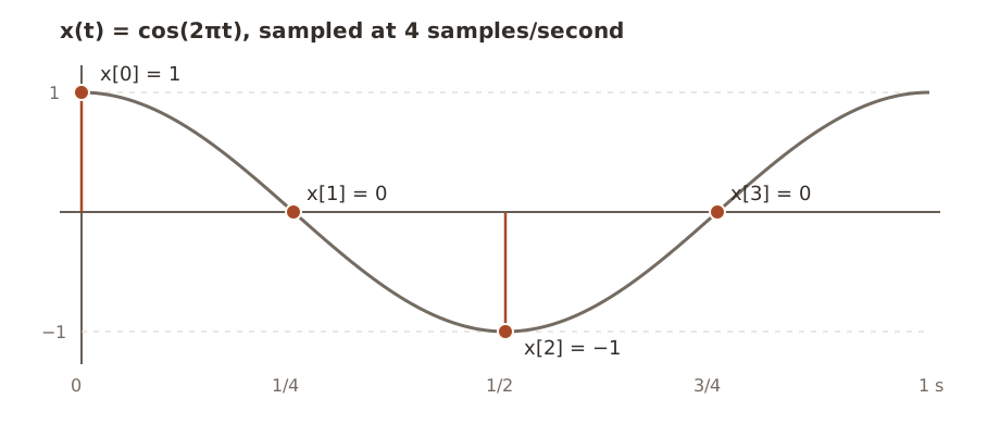
The ratio $f/f_s$ is worth pausing on. The original $f$ tells us cycles per second; dividing by samples per second tells us cycles per sample. It’s the same unit conversion we’ll use when we label the DFT’s frequencies.

Why the DFT uses $k/N$

So far, $f$ has been the frequency of a sinusoid we chose. With a recording, we have the samples and want to find its frequency components. We need to choose some reference sinusoids to test against. The DFT uses a grid of $N$ reference frequencies, called bins.

The candidates are indexed by

$$k=0,1,\ldots,N-1.$$

Candidate $k$ has normalized frequency

$$\boxed{\frac{k}{N}\text{ cycles per sample}}$$

and angular frequency

$$\boxed{\frac{2\pi k}{N}\text{ radians per sample}}.$$

Why choose $k/N$? The useful property is that these reference sinusoids fit a whole number of cycles into one block period. Multiplying the frequency by $N$ sample intervals gives

$$\frac{k\text{ cycles}}{N\text{ samples}} \times N\text{ samples} =k\text{ cycles}.$$

So candidate $k$ completes exactly $k$ cycles per $N$-sample period.

There is one indexing subtlety. The stored samples are $n=0$ through $n=N-1$. The next hypothetical sample, $n=N$, lies on the boundary where the block would repeat. At that boundary, the angle is

$$\frac{2\pi kN}{N}=2\pi k,$$

which lands back at the starting point after $k$ complete turns. This makes the reference sequence repeat every $N$ samples. It doesn’t mean the real recording repeats forever. We’re choosing periodic reference patterns to describe the one block we have.

For $N=8$ and $k=2$, the normalized frequency is

$$\frac{k}{N}=\frac{2}{8}=\frac14\text{ cycle per sample}.$$

Each sample advances by a quarter-turn:

$$0,\ \frac{\pi}{2},\ \pi,\ \frac{3\pi}{2},\ 2\pi,\ldots$$

and the point completes two full turns by the periodic boundary at $n=8$.

To convert the stored bin index into hertz, multiply by the sampling rate:

$$\boxed{f_k=\frac{k}{N}f_s}.$$

The units cancel just as we’d expect:

$$\frac{\text{cycles}}{\text{sample}} \times \frac{\text{samples}}{\text{second}} = \frac{\text{cycles}}{\text{second}}.$$

Adjacent bins are separated by

$$\Delta f=\frac{f_s}{N}\text{ Hz}.$$

At a fixed sampling rate, taking a longer block gives us more closely spaced bins. Its period is $N/f_s$ seconds, even though the elapsed time from the first stored sample to the last is $(N-1)/f_s$ seconds. That final sample interval reaches the next block boundary.

Notice that we chose these frequencies ourselves. We haven’t assumed the input contains only tones that land on the grid. A tone between bins can contribute to several coefficients; we’ll return to that after the worked example.

The candidate complex sinusoids

For each bin $k$, define

$$b_k[n]=e^{j2\pi kn/N}.$$

This is a complex point that advances by $2\pi k/N$ radians whenever $n$ increases by one. It is the $k$-th candidate sinusoid.

• $k=0$ does not rotate. It is the constant sequence $[1,1,\ldots,1]$.
• $k=1$ completes one turn per $N$-sample period.
• $k=2$ completes two turns.
• The pattern continues through $k=N-1$.

We call these basis sequences because we’ll use them as coordinates for the input. The claim is that a weighted sum of these $N$ sequences can reproduce any $N$ samples. In a moment we’ll show why they don’t duplicate one another, which is what makes that claim work.

It’s like describing a diagonal arrow using horizontal and vertical components. The arrow doesn’t have to point along either reference direction. Likewise, our input doesn’t have to look like any single $b_k[n]$.

The DFT as a matching test

We have an arbitrary input $x[n]$ and a candidate rotation $b_k[n]$. We want to measure how strongly they match.

The DFT multiplies the input by the complex conjugate of the candidate and sums over the block:

$$\boxed{ X[k]=\sum_{n=0}^{N-1}x[n]e^{-j2\pi kn/N} }.$$

The complex conjugate of $a+bj$ is $a-bj$, written with a star. It reflects a point across the real axis. Applying that to our candidate gives

$$\left(e^{j2\pi kn/N}\right)^*=e^{-j2\pi kn/N}.$$

Using the positive angles in our definition of $b_k$, the candidate rotates counterclockwise and its conjugate rotates clockwise by the same amount. Why multiply by this opposite rotation? Multiplying complex exponentials adds their exponents, so it gives us a way to subtract the candidate’s angle from the input’s angle.

Suppose the input actually is candidate $k$, with a complex amplitude $C$:

$$x[n]=Ce^{j2\pi kn/N}.$$

Here $C$ is one complex number whose magnitude sets the component’s amplitude and whose angle sets its initial phase.

Multiply by the opposite rotation:

$$\begin{aligned} x[n]e^{-j2\pi kn/N} &=Ce^{j2\pi kn/N}e^{-j2\pi kn/N}\\ &=Ce^0\\ &=C. \end{aligned}$$

Every rotating sample becomes the same stationary complex number $C$. Summing $N$ identical copies gives

$$X[k]=NC.$$

The multiplication is asking:

If I unwind candidate frequency $k$, does part of the signal stop rotating and add in the same direction?

For a matching component, all $N$ contributions point in the same direction instead of cancelling. A different DFT basis frequency leaves a residual rotation whose contributions sum to zero. That exact cancellation is specific to the bin frequencies; an off-grid tone need not cancel completely.

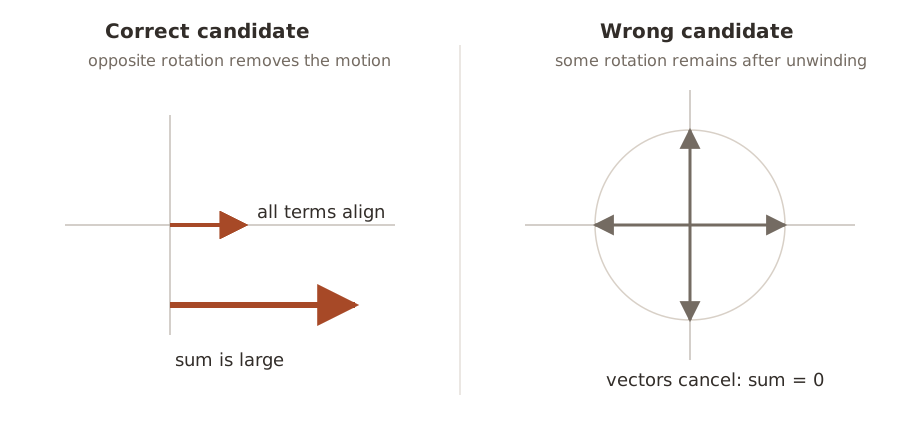
Why wrong frequencies cancel exactly

Let’s check the cancellation rather than relying on the circle picture. Take two bin indices $m$ and $k$, both between $0$ and $N-1$.

Suppose the input contains basis frequency $m$:

$$x[n]=e^{j2\pi mn/N}.$$

Test it against bin $k$:

$$\begin{aligned} X[k] &=\sum_{n=0}^{N-1}e^{j2\pi mn/N}e^{-j2\pi kn/N}\\ &=\sum_{n=0}^{N-1}e^{j2\pi(m-k)n/N}. \end{aligned}$$

If $m=k$, every term is $1$, so the sum is $N$.

If $m\ne k$, there is some rotation left. Depending on the step size, we might visit all $N$ positions around the circle or revisit a smaller set. For example, with $N=4$ and $m-k=2$, the terms are $[1,-1,1,-1]$. They still cancel. To cover every case, let

$$q=e^{j2\pi(m-k)/N}.$$

Then the sum is the geometric series

$$1+q+q^2+\cdots+q^{N-1} =\frac{1-q^N}{1-q}.$$

You can get that fraction by calling the sum $S$, multiplying it by $q$, and subtracting: $S-qS=1-q^N$. All the middle terms cancel. Here $q^N=e^{j2\pi(m-k)}=1$, so the numerator is zero. Our distinct indices lie in $0,\ldots,N-1$, which ensures $q\ne1$. The denominator is therefore nonzero, giving

$$\sum_{n=0}^{N-1}e^{j2\pi(m-k)n/N}=0.$$

Matching bins add to $N$. Different bins add to zero. This is orthogonality, the same idea as the zero dot product between our cosine and sine lists.

It also explains why the DFT works on arbitrary input. An $N$-sample complex list has $N$ complex coordinates. Our $N$ nonzero, mutually orthogonal basis sequences are independent: none can be made by combining the others. They therefore span that whole space, meaning every input has a unique expansion

$$x[n]=\sum_{m=0}^{N-1}C_m b_m[n].$$

Apply the matching test for bin $k$ to this sum. Multiplication and summation distribute over its components. Every term with $m\ne k$ contributes zero, and the term with $m=k$ contributes $NC_k$. So $X[k]=NC_k$, or $C_k=X[k]/N$. This is the coefficient we need to rebuild the input later.

What one coefficient contains

Coming back to real audio samples, what are the two coordinates of $X[k]$? Expand the exponential using Euler’s formula:

$$\begin{aligned} X[k] &=\sum_{n=0}^{N-1}x[n] \left( \cos\left(\frac{2\pi kn}{N}\right) -j\sin\left(\frac{2\pi kn}{N}\right) \right)\\ &=\underbrace{\sum_{n=0}^{N-1}x[n]\cos\left(\frac{2\pi kn}{N}\right)}_{\text{cosine score}}\\ &\quad-j\underbrace{\sum_{n=0}^{N-1}x[n]\sin\left(\frac{2\pi kn}{N}\right)}_{\text{sine score}}. \end{aligned}$$

Write the result as

$$X[k]=R_k+jI_k.$$

Its magnitude is

$$|X[k]|=\sqrt{R_k^2+I_k^2}$$

and its phase is

$$\angle X[k]=\operatorname{atan2}(I_k,R_k).$$

Here $R_k$ is the cosine score and $I_k$ is the negative sine score. Their combined length measures the size of this frequency coefficient. For a real sinusoid on a bin strictly between zero and half the sampling rate, changing the starting phase rotates its coefficient without changing the length. We’ll calculate this explicitly below, including the scaling needed to turn the coefficient’s magnitude into the real wave’s amplitude. The boundary frequencies need separate treatment.

When $|X[k]|=0$, the coefficient is the zero-length arrow, so its phase is undefined. A numerical library may return a conventional value such as zero, but there is no phase to interpret when that frequency has zero magnitude.

Keep track of the minus sign in front of the sine score. It comes directly from $e^{-j\theta}=\cos\theta-j\sin\theta$. The sign and scaling used here match NumPy’s default DFT convention; other conventions are possible if the inverse is changed to match.

We’ve worked out the general test. Let’s now give it four actual numbers and see what comes out.

4. A complete DFT by hand

I’ll use a $1$ Hz cosine sampled four times in one second. A $1$ Hz tone is too slow to hear, but the numbers are easy to follow. Once we’ve done the calculation, we’ll change the time scale to an audible frequency without changing any of the arithmetic.

Step 1: Start with a continuous cosine

Choose a cosine with amplitude $1$, frequency $1$ Hz, and initial phase $0$:

$$x(t)=\cos(2\pi t).$$

It completes one cycle per second and starts at its maximum value.

Step 2: Sample it

Sample at

$$f_s=4\text{ samples per second}$$

and take $N=4$ samples. The sample times are $t_n=n/f_s$.

$n$	$t_n$ in seconds	$x[n]=\cos(2\pi t_n)$
$0$	$0$	$1$
$1$	$1/4$	$0$
$2$	$1/2$	$-1$
$3$	$3/4$	$0$

The DFT receives this list, with no label telling it that the samples came from a cosine:

$$\boxed{x=[1,0,-1,0]}.$$

Step 3: List the four bins

There are $N=4$ bins, so $k=0,1,2,3$. The spacing is

$$\Delta f=\frac{f_s}{N}=\frac44=1\text{ Hz}.$$

Using $kf_s/N$ initially gives $0,1,2,3$ Hz. There’s a sampling ambiguity in that last label, though. At the sample times, adding one full turn per sample has no effect:

$$e^{j2\pi(f/f_s+1)n}=e^{j2\pi(f/f_s)n}e^{j2\pi n}=e^{j2\pi(f/f_s)n}.$$

The last equality holds because $n$ is an integer. In particular, stepping forward by $3/4$ of a turn lands at the same point as stepping backward by $1/4$ of a turn. Bin $3$ can therefore be read as $-1$ Hz. A negative frequency describes clockwise complex rotation; it doesn’t mean a negative number of audible vibrations.

We’ll use these labels:

Bin	Frequency
$k=0$	$0$ Hz, or DC
$k=1$	$+1$ Hz
$k=2$	$2$ Hz, the Nyquist edge
$k=3$	$-1$ Hz

DC means the constant, zero-frequency component. The Nyquist frequency is half the sampling rate, here $2$ Hz. At that frequency, positive and negative rotations both give $[1,-1,1,-1]$, so they share one bin.

For a general $N$, the same wrapping labels upper-half bins with $(k-N)f_s/N$ rather than $kf_s/N$. The lower-half bins keep their positive labels. When $N$ is even, the edge bin $N/2$ can be labeled either $+f_s/2$ or $-f_s/2$; the sample sequence is identical.

Step 4: Test the DC bin, $k=0$

Substitute $k=0$ into the test sequence $e^{-j2\pi kn/N}$:

$$e^{-j2\pi(0)n/4}=[1,1,1,1].$$

Multiply corresponding entries. I’ll use $\odot$ to denote this element-by-element multiplication:

$$[1,0,-1,0]\odot[1,1,1,1]=[1,0,-1,0].$$

Then sum:

$$X[0]=1+0-1+0=0.$$

Since $X[0]$ is the sum of the samples, $X[0]/N$ is their average. Here that average is zero, so we have no constant offset.

Step 5: Test $+1$ Hz, $k=1$

With $k=1$, the test angle steps by $-\pi/2$ each time. At $n=0,1,2,3$, Euler’s formula gives

$$e^{-j2\pi n/4}=[1,-j,-1,j].$$

Multiply:

$$[1,0,-1,0]\odot[1,-j,-1,j]=[1,0,1,0].$$

Sum:

$$\boxed{X[1]=1+0+1+0=2}.$$

Notice what happened at $n=2$: the sample is $-1$ and the test value is also $-1$, so their product is $+1$. The two nonzero products now add instead of cancelling. We have a nonzero $+1$ Hz coefficient, though we still need to explain why its value is $2$ rather than the original amplitude of $1$.

Step 6: Test the Nyquist bin, $k=2$

For $k=2$, the test values alternate between $1$ and $-1$:

$$e^{-j2\pi(2)n/4}=[1,-1,1,-1].$$

Multiply and sum:

$$\begin{aligned} [1,0,-1,0]\odot[1,-1,1,-1]&=[1,0,-1,0],\\ X[2]&=1+0-1+0=0. \end{aligned}$$

The positive and negative products cancel. There is no $2$ Hz basis component in this block.

Step 7: Test $-1$ Hz, $k=3$

For $k=3$, substituting each sample index gives

$$e^{-j2\pi(3)n/4}=[1,j,-1,-j].$$

Multiply and sum:

$$\begin{aligned} [1,0,-1,0]\odot[1,j,-1,-j]&=[1,0,1,0],\\ \boxed{X[3]}&=\boxed{2}. \end{aligned}$$

Another nonzero result, with the same value as bin $1$. Collecting all four sums,

$$\boxed{X=[0,2,0,2]}.$$

Why one real cosine appears in two bins

Our real signal contained one $1$ Hz cosine, so why did both $+1$ Hz and $-1$ Hz respond?

Use Euler’s formula twice:

$$\begin{aligned} e^{j\theta}&=\cos\theta+j\sin\theta,\\ e^{-j\theta}&=\cos\theta-j\sin\theta. \end{aligned}$$

Add them:

$$e^{j\theta}+e^{-j\theta}=2\cos\theta.$$

Therefore

$$\boxed{\cos\theta=\frac12e^{j\theta}+\frac12e^{-j\theta}}.$$

A unit-amplitude real cosine is the sum of two half-amplitude complex rotations, one counterclockwise and one clockwise. At every sample, their imaginary coordinates cancel and their real coordinates add. Earlier we took the real part of a single rotation to obtain a cosine. Here we’re expressing that same cosine as a sum of two rotations, which is the form the DFT uses for reconstruction.

That is why the DFT found a pair:

• $X[1]=2$ represents the positive-frequency rotation;
• $X[3]=2$ represents the negative-frequency rotation.

This pairing holds for any real input, including speech and noise. To see why, conjugate its DFT sum. The samples $x[n]$ stay unchanged because they’re real, while the test exponent changes sign. That is the test for the opposite bin:

$$\begin{aligned} X[k]^*&=\sum_{n=0}^{N-1}x[n]e^{j2\pi kn/N}\\ &=X[N-k],\qquad 1\leq k\leq N-1. \end{aligned}$$

Including $k=0$, we can write it as

$$\boxed{X[(-k)\bmod N]=X[k]^*}.$$

The modulo operation wraps the index into $0,\ldots,N-1$, so the opposite of bin zero is zero itself. This relationship is called conjugate symmetry. Paired magnitudes match, and their phases have opposite signs, up to full turns. For even $N$, we only need to store bins $0$ through $N/2$, or $N/2+1$ coefficients. For odd $N$, we keep $0$ through $(N-1)/2$. The remaining coefficients can be recovered from their partners.

Recover amplitude and phase

For the positive-frequency bin,

$$X[1]=2+j0.$$

Its raw magnitude is

$$|X[1]|=\sqrt{2^2+0^2}=2.$$

Why is the magnitude $2$ when the original cosine’s amplitude was $1$?

Let’s work out both amplitude and phase for a more general cosine. Suppose it lands exactly on a positive-frequency bin $k$, with $0<k<N/2$:

$$x[n]=A\cos\left(\frac{2\pi kn}{N}+\phi\right).$$

Using the two-rotation identity,

$$x[n]=\frac{A}{2}e^{j\phi}e^{j2\pi kn/N} +\frac{A}{2}e^{-j\phi}e^{-j2\pi kn/N}.$$

The coefficient of the positive rotation is $(A/2)e^{j\phi}$. Testing bin $k$ leaves that number stationary for all $N$ samples. The negative rotation is a different basis frequency, so its contribution to this test cancels. We therefore get

$$X[k]=\frac{NA}{2}e^{j\phi} =\frac{NA}{2}\cos\phi+j\frac{NA}{2}\sin\phi.$$

This explains both parts of the answer. The arrow has length $NA/2$ and angle $\phi$. The factor $N$ came from summing $N$ identical contributions; the factor $1/2$ came from splitting the cosine between two rotations. Solving for $A$ gives

$$\boxed{A=\frac{2|X[k]|}{N}}.$$

In our example,

$$A=\frac{2(2)}{4}=1.$$

This amplitude formula assumes the unscaled forward DFT we’ve used, a bin-centered cosine, and no tapering window applied to the samples. It isn’t a general rule for reading any physical tone’s amplitude from the nearest peak. We’ll look at what changes when a tone falls between bins in the audio section.

DC and, for even $N$, Nyquist have no separate conjugate partners, so we don’t double them. The signed constant level is $X[0]/N$. The coefficient $X[N/2]/N$ multiplies the alternating sequence $(-1)^n$. These boundary bins don’t provide the same two-coordinate phase measurement as an interior positive-frequency bin.

The phase is the coefficient’s angle:

$$\phi=\angle X[1]=\operatorname{atan2}(0,2)=0.$$

This is the initial phase relative to sample $n=0$, not the changing angle of the wave at every subsequent sample. If the coefficient were zero, there would be no angle to recover.

So the DFT recovered

$$\boxed{f=1\text{ Hz},\qquad A=1,\qquad \phi=0}.$$

The same frequency at three phases

It’s easy to miss the role of phase when every result is real. Let’s keep the frequency and amplitude fixed and shift the wave’s starting point:

Real signal	Samples	$X[1]$	Raw magnitude	Phase
$\cos(2\pi n/4)$	$[1,0,-1,0]$	$2+j0$	$2$	$0$
$\cos(2\pi n/4+\pi/2)$	$[0,-1,0,1]$	$0+j2$	$2$	$+\pi/2$
$\sin(2\pi n/4)$	$[0,1,0,-1]$	$0-j2$	$2$	$-\pi/2$

The last line uses

$$\sin\theta=\cos\left(\theta-\frac{\pi}{2}\right).$$

For the sine in the last row, the cosine score is zero and the sine score is $2$, just as we calculated earlier. The DFT combines them as $0-j2$, so its angle is $-\pi/2$. That agrees with the cosine form of sine above. Using $+j$ times the sine score here would give the wrong phase for our convention.

All three coefficients have length $2$, which converts to real amplitude $1$ after multiplying by $2/N$. Their angles differ because the waves start at different points in the cycle. If we threw away those angles and kept only magnitudes, we couldn’t tell these three sample lists apart.

We can check the whole phase relationship without choosing a particular angle. Four samples of $A\cos(2\pi n/4+\phi)$ are

$$A[\cos\phi,-\sin\phi,-\cos\phi,\sin\phi].$$

Multiply by the bin-$1$ test $[1,-j,-1,j]$ and sum:

$$\begin{aligned} X[1]&=A\cos\phi+jA\sin\phi\\ &\quad+A\cos\phi+jA\sin\phi\\ &=2Ae^{j\phi}. \end{aligned}$$

Changing $\phi$ rotates this coefficient. Changing $A$ changes its length. The two numbers in a complex coefficient are doing separate, measurable jobs.

Reconstruct the samples with the inverse DFT

The inverse DFT is

$$\boxed{ x[n]=\frac1N\sum_{k=0}^{N-1}X[k]e^{j2\pi kn/N} }.$$

We already found the reason for this formula: each basis weight is $C_k=X[k]/N$. Multiply each original basis sequence by its weight and add them. That’s why the exponent is positive again and why the sum has a factor of $1/N$.

For our example, only $X[1]$ and $X[3]$ are nonzero:

$$x[n]=\frac14\left(2e^{j2\pi n/4}+2e^{j2\pi(3)n/4}\right).$$

Bin $3$ is the $-1$ Hz rotation, so this is

$$x[n]=\frac12\left(e^{j2\pi n/4}+e^{-j2\pi n/4}\right).$$

Using the identity we derived earlier,

$$x[n]=\cos\left(\frac{2\pi n}{4}\right).$$

If we check each position before cancelling the imaginary parts, the reconstruction is

$n$	Positive rotation’s contribution	Negative rotation’s contribution	Sum
$0$	$1/2$	$1/2$	$1$
$1$	$j/2$	$-j/2$	$0$
$2$	$-1/2$	$-1/2$	$-1$
$3$	$-j/2$	$j/2$	$0$

So the inverse gives us

$$\boxed{x=[1,0,-1,0]},$$

exactly the samples we started with.

Why spend this much time on four numbers? They let us check everything the DFT claims to do: identify a matching frequency, reject the other basis frequencies, recover amplitude and phase, and reconstruct the input. A software library does the same calculation on a larger block, where writing out every product would be impractical.

We can also make this an audible example without changing the list. Sample a $1{,}000$ Hz cosine at $4{,}000$ samples per second and take four samples. The ratio $f/f_s$ is still $1/4$, so the input remains $[1,0,-1,0]$ and its DFT remains $[0,2,0,2]$. Bin $1$ now means $1{,}000$ Hz. The sample values determine the DFT coefficients; the sampling rate tells us how to label them in hertz.

5. Return to real audio

What if the samples are not a sinusoid?

They usually aren’t. Speech and music contain overlapping components, and their amplitudes and frequencies can change while we’re recording. But we’ve already shown that the $N$ basis sequences span the space of all $N$-sample lists. The samples don’t need to come from a single pure tone.

There’s another useful consequence of the multiply-and-sum formula: the DFT of a sum of signals is the sum of their DFTs. If we add a second tone to our first, its coefficients are added to the result. This property is called linearity.

Take the opening example: a cosine at $440$ Hz with amplitude $1$, plus one at $880$ Hz with amplitude $0.25$, both starting at phase zero. Sample at $48{,}000$ Hz and take $N=4{,}800$ samples. The bin spacing is $10$ Hz, so the tones land exactly on bins $44$ and $88$.

From $X[k]=NA/2$ for these zero-phase cosines, the positive-frequency coefficients are

$$X[44]=2400,\qquad X[88]=600.$$

Their negative-frequency partners are bins $4756$ and $4712$, with the same values. All other coefficients are zero in exact arithmetic. We can recover the two amplitudes as $2(2400)/4800=1$ and $2(600)/4800=0.25$, even though we fed the DFT the sum of the two waves. The four-sample example scales directly to a mixture at audible frequencies.

This is useful for more than drawing a spectrum. Suppose we multiply both $880$ Hz coefficients by $1/2$ and take the inverse DFT. We get the same $440$ Hz component and an $880$ Hz component with amplitude $0.125$. We’ve changed the balance of the sound by changing two numbers. We adjust both partners so that the reconstructed samples remain real.

An equalizer extends this idea to ranges of frequencies. In practical audio processing, handling block boundaries also matters; abruptly editing and joining independent blocks can introduce artifacts. But the reason to work in frequency coordinates is already visible in this example. They let us address parts of a signal that are mixed together in the waveform.

Other uses include:

• Looking for harmonics: peaks at a fundamental frequency and its integer multiples, like $440$ and $880$ Hz.
• Locating a persistent hum or a broad band of noise in a recording.
• Measuring spectral patterns that help distinguish instruments or speech sounds. The largest peak alone need not be the perceived pitch.

What if a sound changes during the block? The full complex DFT still contains enough information to reconstruct those changes, but a single magnitude plot has no time axis. It doesn’t directly show us when a tone appeared. For that view, we take short, usually overlapping blocks, apply a window to each, and compute their DFTs. This is the Short-Time Fourier Transform (STFT). Plotting magnitude or squared magnitude against both time and frequency gives a spectrogram, often displayed on a logarithmic scale.

Practical details the clean example hides

The arithmetic above was exact because we chose tones that fit the bins. With an actual recording, there’s a difference between reconstructing the samples and identifying the physical sounds that produced them. The DFT always gives us the former. These are some things to account for when attempting the latter.

Bin spacing and observation length

The distance between bins is

$$\Delta f=\frac{f_s}{N}.$$

Our $4{,}800$ samples at $48{,}000$ Hz cover a block duration of $0.1$ seconds, giving bins $10$ Hz apart. Recording twice as long gives bins $5$ Hz apart. But a longer block also combines more of the sound’s evolution into one spectrum. That’s the tradeoff when choosing a frame length for a spectrogram: short frames help locate changes in time, while long frames help separate nearby tones. Bin spacing alone isn’t the full measure of how well we can separate tones; the window and noise also matter.

Spectral leakage

What if we replace the $440$ Hz tone with $443$ Hz? In a $0.1$ second block it completes $44.3$ cycles, so none of our integer-cycle basis sequences matches it exactly. Its DFT generally has contributions across many bins, strongest near the tone. This spreading is called spectral leakage. The reconstruction is still exact; it just takes more basis components to represent those samples.

Repeating the block helps explain this. An off-grid sinusoid generally doesn’t continue smoothly when we restart the recorded segment, so its periodic extension needs additional frequencies. Be careful with the endpoints here: we don’t require the last stored sample to equal the first. Our leakage-free cosine $[1,0,-1,0]$ didn’t satisfy that either. The first sample of the next period comes one sample interval after the last stored sample.

A window is a list of weights $w[n]$ applied before the DFT, so we transform $w[n]x[n]$. A tapering window gives less weight to the ends of the block. Common choices reduce distant leakage at the cost of widening the central peak. They also change amplitude scaling, so our earlier $2|X[k]|/N$ shortcut no longer applies unchanged. SciPy’s spectral analysis tutorial shows these window and scaling tradeoffs in more detail.

Aliasing and the Nyquist limit

After sampling, frequencies separated by an integer multiple of $f_s$ produce the same samples. We therefore cannot distinguish every possible continuous frequency from discrete samples alone.

For real audio, we conventionally show nonnegative frequencies up to the Nyquist frequency,

$$f_{\mathrm{Nyquist}}=\frac{f_s}{2}.$$

The negative-frequency half is determined by conjugate symmetry. But that redundancy doesn’t prove that the analog sound contained only frequencies below $f_s/2$. A higher-frequency tone can produce exactly the same samples as a lower one. This ambiguity is aliasing, and the DFT cannot undo it.

For example, at $f_s=4$ samples per second, $\cos(2\pi t)$ and $\cos(2\pi\cdot3t)$ both give $[1,0,-1,0]$ at our four sample times. We know which signal we used in the worked example because we chose it. The DFT alone can’t make that distinction.

This is why recording systems use an anti-aliasing filter before sampling, to suppress frequencies outside the intended band. In the ideal sampling theorem, a signal band-limited strictly below $f_s/2$ can be recovered from its complete, exact sample sequence. “Band-limited” here means it has no frequency content at or above that limit in absolute frequency. A finite block of rounded ADC values is a more limited observation. MIT’s notes on sampling and reconstruction develop this distinction further.

The strict boundary matters. At exactly $f_s/2$, a sine with zero initial phase gives $\sin(\pi n)=0$ at every sample. Its continuous oscillation vanishes from the recorded sequence. We shouldn’t use the Nyquist bin to infer an arbitrary analog sinusoid’s amplitude and phase as though it were an interior bin.

Magnitude, power, and phase are different views

For a coefficient $X[k]$:

$$\begin{aligned} \text{raw magnitude}&=|X[k]|,\\ \text{raw squared magnitude}&=|X[k]|^2,\\ \text{phase}&=\angle X[k]. \end{aligned}$$

Magnitude measures coefficient size. Squared magnitude is related to signal energy: with our DFT convention, the block’s mean-square sample value is $\frac{1}{N^2}\sum_k|X[k]|^2$, summing all $N$ bins. Converting that to physical power requires knowing what the sample values represent. A power spectral density additionally describes power per unit frequency, so its normalization involves frequency spacing and, when used, the window.

Phase carries alignment information. Our three phase-shifted four-sample signals had identical magnitude spectra but different samples. A magnitude-only plot is useful for seeing prominent frequencies, but those magnitudes alone aren’t enough to reconstruct the sound.

Zero-padding does not create new resolution

We could append zeros to our $4{,}800$ measured samples and compute a larger DFT. That evaluates the same finite recording’s DTFT at more closely spaced frequencies. The plot becomes smoother and a peak may be easier to locate, but we haven’t listened to any more sound. Closely spaced tones that were unresolved in the original observation don’t become separable merely because we drew more points. This MathWorks example illustrates what zero-padding can do for amplitude estimation.

All of these details affect how we interpret a spectrum. None prevents the inverse DFT from reconstructing the finite list we actually transformed. If we tapered it first, that list is the windowed samples; if we padded it, it includes the appended zeros.

6. The whole DFT in one pass

Coming back to the formula at the start of the post,

$$X[k]=\sum_{n=0}^{N-1}x[n]e^{-j2\pi kn/N}.$$

1. Choose a frequency bin $k$.
2. At each sample $n$, evaluate the opposite-rotation test $e^{-j2\pi kn/N}$.
3. Multiply that complex point by the real sample value $x[n]$.
4. Sum all $N$ results.
5. Read the resulting complex number $X[k]$. Its length gives the coefficient magnitude; its angle gives the component’s initial phase when that magnitude is nonzero. Convert to real sinusoid amplitude using the appropriate scaling.
6. Repeat for all $k=0,1,\ldots,N-1$.

The inverse DFT takes those coefficients, rebuilds every basis rotation, and adds them to recover the samples.

The two views agree. Multiplying and summing measures the basis weights; adding the weighted basis sequences reconstructs the input. That’s why the same transform can help us inspect a recording and then edit it.

7. From the DFT to the FFT

If we wrote code that followed our hand calculation literally, we’d loop over the samples once for every bin. For each new bin we’d calculate another set of rotations and another sum.

The direct formula computes $N$ terms for each of $N$ bins. That requires work proportional to

$$N^2.$$

With $N=1{,}024$, that’s $1{,}048{,}576$ sample-times-test terms for a single transform. If we’re processing overlapping audio frames continuously, that work adds up.

But those rotations aren’t unrelated. We’ve already used the fact that powers of $j$ repeat and that adding full turns leaves the sample values unchanged. The Fast Fourier Transform (FFT) uses symmetries in the DFT to reuse work across bins, reducing the cost to order

$$N\log N.$$

The mathematical result is the same DFT. An FFT changes how we calculate the coefficients, with ordinary floating-point rounding in a numerical implementation. We don’t give up frequency bins or discard phase to get the speedup.

The next post will start by splitting the samples into even and odd indices. That gives us two smaller DFTs. The interesting question is how to combine them without doing all the work again, and the answer comes from the same complex rotations we’ve been using throughout this post.

References

• NumPy’s DFT conventions and implementation notes
• MIT OpenCourseWare notes on sampling and the DFT
• MathWorks example on zero-padding and frequency resolution
• SciPy’s tutorial on spectral analysis, windows, and scaling
• Cooley and Tukey’s 1965 FFT paper