Concentration of Measure

I recently wrote a piece about the increasing polarization of the general public and why I believe it has a statistical basis in the sharp uptick in the number of opinions the average person is expected to hold. You can find that post here. I wanted to formalize the math behind the intuition here on the blog where LaTeX is first-class.

There’s certain holes in my reasoning below that I’m still trying to make sense of. The ones I’m aware of I’ve elucidated; the others I hope will come in the form of feedback. Suggestions and corrections are always welcome.

We want to show that most randomly sampled Gaussian vectors in high dimensional spaces aren’t close to the center of the distribution but rather lie some distance away from the center. We also want to show what this distance is. I want to outline two possible approaches and show how they converge to (nearly) the same result:

1. Transformations between probability distributions combined with some neat tricks from convex optimization.
2. Brute force calculus.

Approach 1

Objective: Show that a randomly sampled vector from an $n$ dimensional standard Gaussian will on average be $\sqrt{n}$ units of distance away from the origin.

Proof: Consider a random vector $\mathbf{X}$ sampled from a multivariate standard Gaussian.

$$\mathbf{X} \sim \mathcal{N}(\boldsymbol{\mu}, \boldsymbol{\Sigma}), \quad \boldsymbol{\mu} = \mathbf{0} \quad \boldsymbol{\Sigma} = \mathbf{I}$$

We define $\boldsymbol{\Sigma}$ as the identity covariance matrix in $\mathbb{R}^n$ and $\boldsymbol{\mu}$ as the zero vector. Each element of $\mathbf{X}$ is drawn from the univariate standard normal distribution:

$$x \sim \mathcal{N}(0, 1)$$

Consider the squared length of this vector $\mathbf{X}$ (length here refers to the L2 norm). We can write out this expression as:

$$\|\mathbf{X}\|_2^2 = x_1^2 + x_2^2 + \ldots + x_n^2$$

The expected value for this expression is intuitively the average squared length of the random vector $X_i$ drawn from $\mathbf{X}$.

$$E[\|\mathbf{X}\|_2^2] = E[x_1^2 + x_2^2 + \ldots + x_n^2] = E\left[\sum_{i=1}^{n} x_i^2\right]$$

By linearity of expectation, we obtain the following:

$$E[\|\mathbf{X}\|_2^2] = \sum_{i=1}^{n} E[x_i^2]$$

Recall that each $x_i$ is a univariate standard normal random variable. It is a well-known fact that squaring a Gaussian random variable in $n$ dimensions transforms it into a random variable sampled from a chi-squared distribution with $n$ degrees of freedom. This gives us the distribution of each $x_i^2$ term:

$$x^2 \sim \chi^2(1, 2)$$

The above expression tells us the mean of the univariate chi-squared distribution is just 1 which means each term in the earlier summation equals 1.

$$E[\|\mathbf{X}\|_2^2] = E[x_1^2 + x_2^2 + \ldots + x_n^2] = \sum_{i=1}^{n} E[x_i^2] = \sum_{i=1}^{n} 1 = n$$

Conclusion: The average squared length of a vector in $n$ dimensions is then just equal to $n$. Take a second here to work through the argument above and convince yourself why this is true.

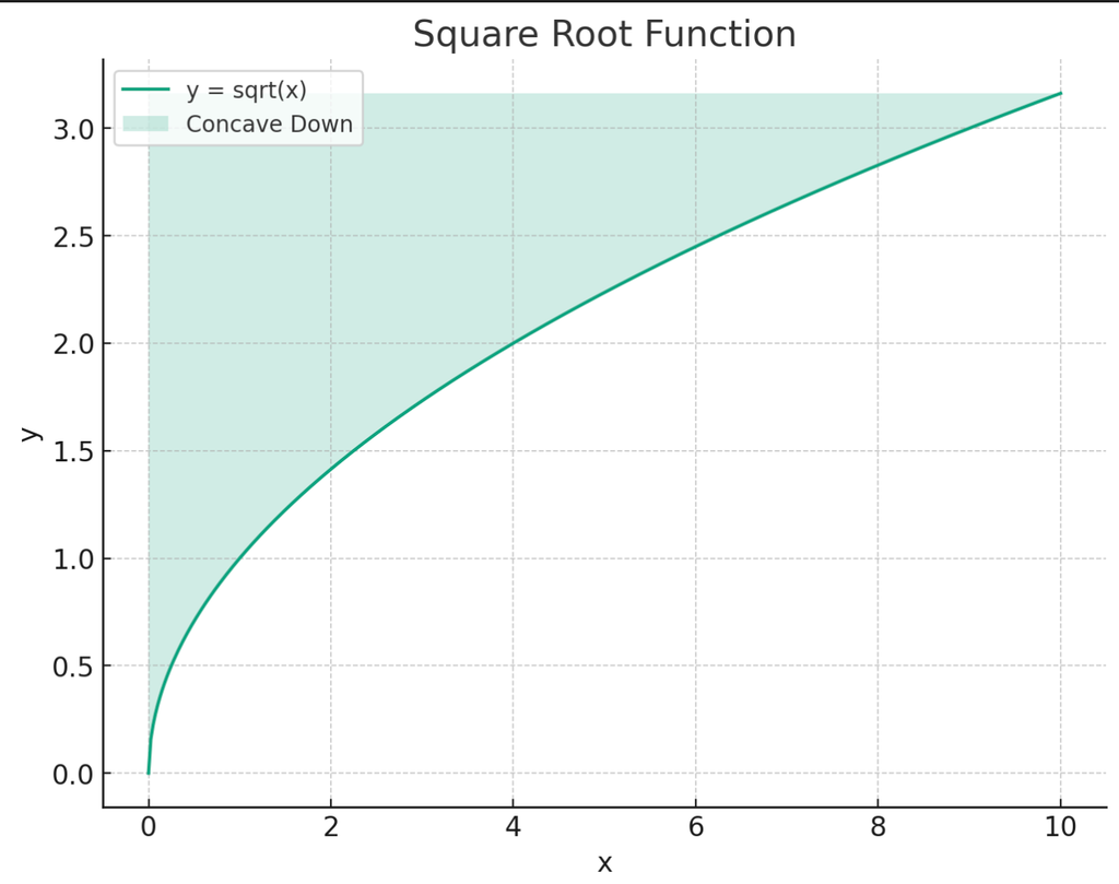
But we’re not done yet. Our objective was to determine the average length, not the average squared length. It might be tempting to just take the square root of the answer above. But remember that the square root is a non-linear concave function so linearity of expectation doesn’t apply.

Luckily we can turn to Jensen’s inequality which tells us that for a concave function $g$ and a random variable $Y$:

$$E[g(Y)] \leq g(E[Y])$$

In the context of our problem, we can plug in the square root function as $g$ and the chi-squared random variable as $Y$ to get:

$$E[\sqrt{\|\mathbf{X}\|_2^2}] \leq \sqrt{E[\|\mathbf{X}\|_2^2]} \quad \Rightarrow \quad E[\|\mathbf{X}\|_2] \leq \sqrt{n}$$

The term on the left is what we want (the expected value of the length) whereas the term on the right is what we would get if we naively took the square root of the mean of the chi-squared random variable.

The inequality above tells us that the term on the right is an upper bound on our actual desired value on the left. But we can do better than just an upper bound.

The expected value of a random variable $f(X)$ can be found by integrating the function $f$ over the probability density function of the random variable $X$ over the domain of $X$.

$$E[f(X)] = \int_{0}^{\infty} f(x) \cdot p_{x;k} \, dx$$

Let’s plug our expression in. The expression we want to evaluate is:

$$E[\sqrt{\|\mathbf{X}\|_2^2}]$$

$f$ is the square root function and $p_{x;k}$ is the PDF of the chi-squared distribution with $k$ degrees of freedom.

$$E[\sqrt{\|\mathbf{x}\|_2^2}] = \int_{0}^{\infty} \sqrt{x} \cdot \frac{1}{2^{n/2} \Gamma(n/2)} x^{(n/2 - 1)} e^{-x/2} \, dx$$

where $\Gamma$ is the gamma function.

Recall that the gamma function is the generalization of the factorial to complex numbers. While this integral doesn’t have a simple closed form solution, we can leverage numerical integration methods to evaluate it at specific values of $n$ and compare it to our naive solution of $\sqrt{n}$. Here’s what that graph looks like plotted across a range of dimensions (x-axis).

We’ve numerically verified Jensen’s inequality to hold true. The solid green line representing $f(E[X])$ is indeed always below the dotted line representing $E[f(X)]$. But the most interesting observation is that the two lines converge! Which means as we scale the dimensionality of our space, the average length of a vector converges to our naive solution of $\sqrt{n}$.

Approach 2

In the previous section we tried to answer the question: “What is the average distance from the origin for a randomly sampled vector in $n$ dimensions?”

But we can also formulate an alternate question: “At what distance from the origin does the probability of finding a vector take its maximum value?”

This framing reduces our question to a simple optimization problem. All we need now is an objective function to maximize. So let’s derive that.

We know that working with continuous distributions entails dealing with probability density functions (PDFs) as opposed to discrete distributions where we deal with probability mass functions (PMFs). When I first studied the two I didn’t pay too much attention to why they were named different things. The only difference I cared about was how you read them:

1. The y-axis on the graph of a PMF shows probabilities.
2. The y-axis on the graph of a PDF does not show probabilities: you need to integrate under the curve if you want that.

This difference is not just convention; the reason for it can be found simply by looking at the two names.

When we measure probabilities on the y-axis of a PMF, what we are really measuring is probability mass. A PDF does not show probabilities on the y-axis because it is not a measure of mass but rather of density. Forget about probabilities for a second and consider density as we apply it to physical quantities. The density of a substance is measured as the mass of that substance per unit volume. To get the mass of a substance, you need to multiply its mass by the volume it occupies. If you extend the volume over an interval, this “multiplication” is just integrating the product of density and volume over that interval. Which is exactly what we do when trying to obtain probability masses from a PDF!

The probability density $p_{x;n}$ of a multivariate standard Gaussian in $n$ dimensions is given by the following expression:

$$p(\mathbf{x}) = \frac{1}{(2\pi)^{n/2}} \exp\left(-\frac{1}{2} \mathbf{x}^T \mathbf{x}\right)$$

For any given $\mathbf{X}$, we can make a simplifying observation: the value of the PDF depends only on the magnitude of $\mathbf{X}$ and not on the actual direction of $\mathbf{X}$. We know this because the only dependency on $\mathbf{X}$ in the above expressions comes from the $\mathbf{X}^T\mathbf{X}$ term — this is just the squared magnitude of $\mathbf{X}$.

Let $R$ be the magnitude of $\mathbf{X}$. We can then make the substitution $\mathbf{X}^T\mathbf{X} = \|\mathbf{X}\|_2^2 = R^2$. This gives us:

$$p(\mathbf{x}) = \frac{1}{(2\pi)^{n/2}} \exp\left(-\frac{1}{2} R^2\right)$$

This gives us exactly what we need: an expression in terms of $R$ (the magnitude of the vector which is equivalent to the distance of the vector from the origin). Our objective is going to be to find the value of $R$ for which the product of the density and volume functions is maximized.

Now we need an expression for the volume. The first question to answer is what shape are we modeling the volume off?

The volume of the amount of space present at a distance $R$ from the origin in an $n$ dimensional space can be thought of as the volume of an $n$ dimensional hypersphere with radius $R$. To convince yourself of why this might be true, look at the expression for the probability density and our observation about how the density is affected by different $\mathbf{X}$‘s. For $\mathbf{X}_i$‘s in different directions, as long as they have the same magnitude, the PDF evaluates to the exact same value. If you imagine taking a set of $\mathbf{X}_i$‘s that are all pointing in different directions but have the same distance from the center, all of them evaluate to the same value when plugged into the PDF. A circle is defined as a collection of points in a plane that are all equidistant from a reference point. We can then think of each unique magnitude of the $\mathbf{X}$‘s as defining a unique contour circle — every $\mathbf{X}$ along a contour circle has the exact same magnitude and hence the exact same density.

This is slightly less intuitive so let’s start from the two dimensional case and build upwards.

The volume of a sphere in 2D (a circle) is just its surface area: $4\pi R^2$.

The volume of a sphere in 3D (what we think of as a sphere) is given by: $\frac{4}{3}\pi R^3$.

The generalization of the volume of a hypersphere in $n$ dimensions is given by the expression:

$$V_n = \frac{\pi^{n/2}}{\Gamma(\frac{n}{2} + 1)} R^n$$

One way to intuitively grasp the above expression is that it represents the space in which our probability mass lives. It might be tempting at this point to directly multiply our expression for the volume by the expression for density and optimize the result. But we can’t use the above expression directly. We are interested in finding the distance $R$ at which the probability mass is maximized. But this requires us to know the mass concentrated exactly at that distance, not all the mass up to and including that distance. In other words, we don’t want to know how much mass is concentrated inside a hypersphere of radius $R$; we want to know how much mass is concentrated at an infinitesimally thin shell exactly at the radius $R$.

We can think of this as the product not between density and volume but rather between density and differential volume. This is just the derivative of the above expression with respect to $R$:

$$dV_n = \frac{\pi^{n/2}}{\Gamma(\frac{n}{2} + 1)} n R^{n-1} \, dR$$

Take a second here to understand why we are using the differential volume. We know that probability density is different at different parts of the sphere depending on how far out you are (the value of $R$). To know the value of the probability mass at any of these distances, we need to know the density per unit volume. The unit volume here can be thought of as an increasingly thin shell at that distance $R$. The limit as this shell approaches 0 is just the definition of the derivative of the volume function!

Let’s compare the two expressions for density and volume.

Density at distance $R$:

$$\frac{1}{(2\pi)^{n/2}} \exp\left(-\frac{1}{2} R^2\right)$$

Differential volume at distance $R$:

$$\frac{\pi^{n/2}}{\Gamma(\frac{n}{2} + 1)} n R^{n-1} \, dR$$

What do you notice about the behavior of each of these functions?

Density is monotonically decreasing — in fact exponentially decaying in proportion to $O(R^2)$. As $R$ gets larger, density starts dropping and the rate at which it drops gets faster as $R$ increases.

Differential volume on the other hand is monotonically increasing — in fact polynomially growing in proportion to $O(R^n)$.

These two insights form the final piece of our intuition for why probabilities behave differently in higher dimensions. In lower dimensions, all we think about are the density curves. But in higher dimensions, volume is just as important because there is just so much more space to occupy.

Think about moving from 1D to 2D to 3D. Each time you move up a dimension, you add an entirely new axis of movement. An axis that is orthogonal to the others and could never have been reached from a combination of the previous ones. A being that can move in 3D space can access infinitely more space than a being restricted to move along two dimensions. Just by adding a single new dimension of movement. That increase in freedom happens every single time you add a dimension, even though we can’t picture anything above three dimensions.

Coming back to our expressions, we see that for higher values of $n$, the growth of differential volume outpaces the exponential decay of density for a longer period of time. Eventually there is always a point where the rate at which density falls starts outpacing the rate at which volume grows but the distance from the origin at which that cross-over happens gets pushed out further and further the higher up you go in the dimensions.

The graphs below showcase this phenomenon. The x-axis are values of $R$ moving out farther from the origin. The blue line represents the density function evaluated at those values of $R$, the green line represents the differential volume present at that distance, and the red line represents the product we are interested in. We plot this out for a range of $n$ values.

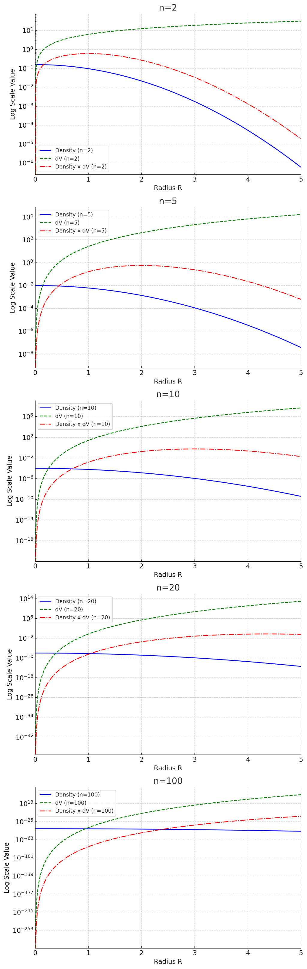
Notice that as $n$ increases, the maximum value of the product between density and volume gets pushed out to increasingly higher values of $R$. The maximum is reached when the magnitude of the derivative of the density function (the rate of density decay) exceeds the magnitude of the derivative of the differential volume (the rate of volume growth).

Now all that’s left is to derive a closed form expression for where this maximum lies. To do this, we first write out the product of the differential volume and the density:

$$m_r = \frac{2^{1 - \frac{D}{2}} R^{D - 1} \exp\left(-\frac{R^2}{2}\right)}{\Gamma\left(\frac{D}{2}\right)}$$

where $m_r$ = differential mass at radius $R$.

We then take the derivative of this expression with respect to $R$, set it to 0, and solve for $R$:

$$\frac{dm_r}{dR} = 0$$

A little help from sympy and we’re left with the following critical point for the maximum:

$$R = \sqrt{n - 1}$$

Therefore in $n$ dimensions, the annulus containing the most probability mass can be found at a distance of $\sqrt{n - 1}$ from the origin. Let’s see what this looks like across different dimensions.

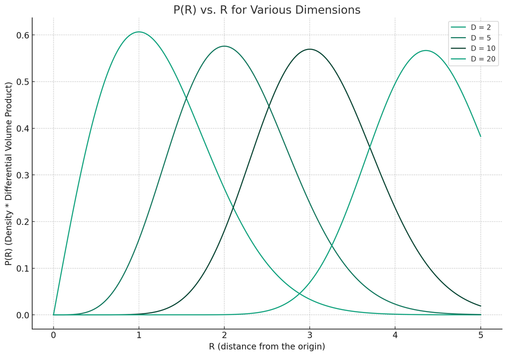
The peak of the density × differential volume, representing the maximum value of the probability mass across all possible shell radii, shifts to the right as the dimension increases.

Here’s the visualization that really blows our intuition out of the water: for all these dimensions, the peak of the PDF would still be centered at 0!

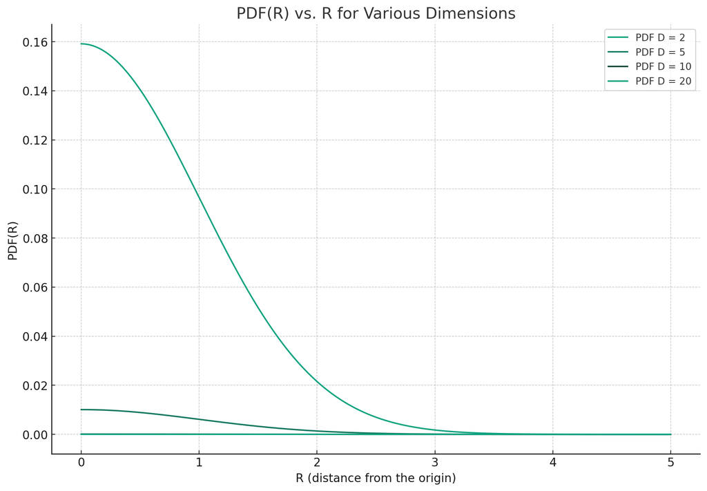
All of the PDFs peak at 0 and exponentially decay as $R$ increases. This is why simply analyzing PDFs or probability densities in high dimensions can be so misleading — highest density no longer corresponds to greatest mass.

Some appendix thoughts on the two answers of $\sqrt{n}$ and $\sqrt{n - 1}$.

That discrepancy between Approach 1 and 2 bothers me but I can’t seem to formalize the difference. Any suggestions here would be invaluable.

The intuitive argument I’d make is that Approach 1 provides an expected value over the magnitude of $\mathbf{X}$ whereas Approach 2 provides a single extremum at which the probability mass is maximized. These two aren’t equivalent. The easiest way to see this is in the 1 dimensional case. The expected value suggests that most vectors (points) in the 1D Gaussian would be found at a distance of 1 which is clearly not the peak of the density function. But that is because we are not taking the expectation over the Gaussian random variables themselves but rather just their magnitude. The magnitudes of all points sampled from the Gaussian are positive so it makes sense that their mean isn’t centered at 0 but rather around 1. This also makes sense once you realize that the standard deviation of the standard Gaussian is also (coincidentally?) 1 so we’re really measuring a spread of distance from the origin with the expected value of the magnitude.